A comprehensive review of computer architecture.
The course textbook is Computer Organization and Design: The Hardware/Software Interface, 6th Edition.
References:
- CAAQA (Computer Architecture: A Quantitative Approach; please use a legitimate copy of the textbook)
- Official RISC-V specifications
Introduction
What is computer architecture?
Maximizing machine performance for the specific needs of the target machine, under constraints such as cost, power, and availability. It covers the ISA, computer organization (microarchitecture), and hardware implementation.
Key Design Ideas
- Abstraction
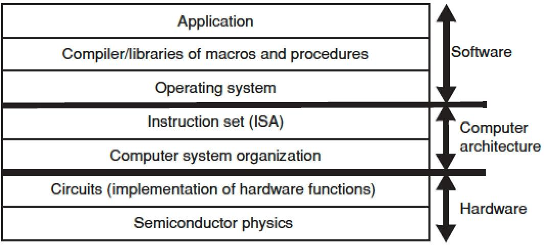
- Layered design: application → compiler → OS → ISA → hardware circuits
- Key value: simplifies the design of complex systems (e.g., the instruction-set abstraction)
Moore’s Law
- Original statement (1965): transistor density doubles every 1–2 years
- Modern challenges:
- 3D stacking (e.g., the Cerebras wafer-scale chip with 1.2 trillion transistors)
- Chiplet technology (used in AMD GPUs to address yield problems)
- Power wall: physical limits caused by excessive power density on the chip
Principle of Locality and the Memory Hierarchy
- Memory pyramid: registers → L1/L2/L3 cache → main memory → virtual memory → disk
Dependability via Redundancy
- Example: ECC memory (9 chips vs. 8 chips for non-ECC; the redundant chip corrects errors)
Parallelism
- Levels:
- Instruction-level (ILP): pipelining, out-of-order execution
- Data-level (DLP): SIMD/vector processors
- Task-level (TLP): multithreading/multicore
- Levels:
Representation and Computation of Data
Von Neumann Architecture and Harvard Architecture
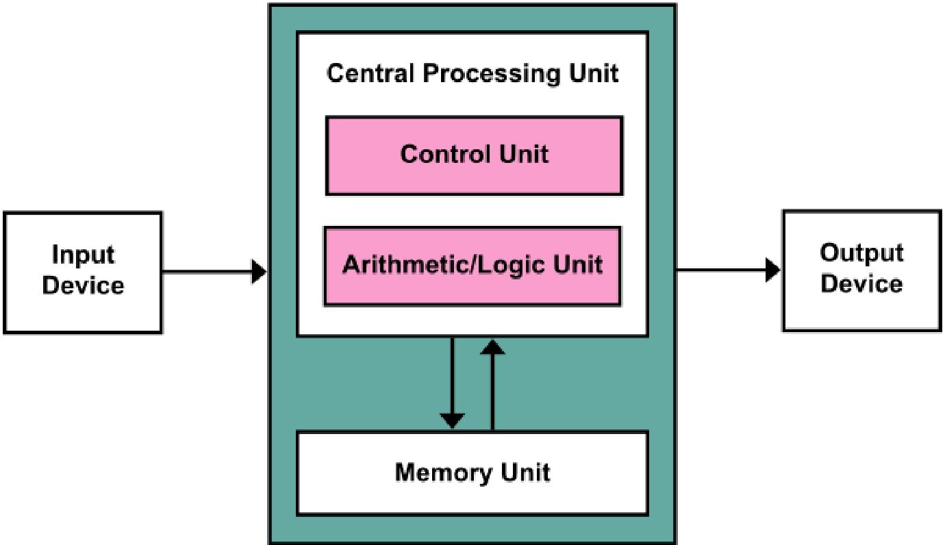
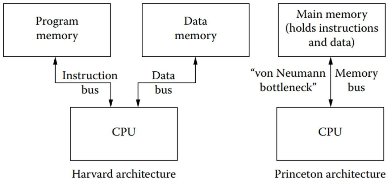
- Von Neumann architecture: stored program; data and instructions share the same memory
- Harvard architecture: data and instructions are stored separately; commonly used in embedded systems
Sign-Magnitude, Ones’ Complement, and Two’s Complement
- Sign-magnitude: sign bit + absolute value
- Ones’ complement (1’s complement): sign bit unchanged; for negative numbers, invert the remaining bits
- Two’s complement (2’s complement): sign bit unchanged; for negative numbers, invert the bits and add 1
- unsigned extension: pad the high bits with 0
- signed extension: pad the high bits with the sign bit
- Type conversion: arithmetic between int and unsigned is converted to unsigned
Ripple-Carry Adder
- Full adder: inputs A, B, Cin; outputs Sum and Cout
- Ripple-Carry Adder: multiple full adders chained in series to compute the sum A+B+C
- Delay: each full adder has a delay of 1, so n full adders have a total delay of n
- Overflow detection: for an n-bit two’s complement adder, overflow occurs if A and B have the same sign bit and it differs from the sign bit of Sum
IEEE 754 Floating Point
- Single precision: 1 sign bit, 8 exponent bits, 23 mantissa bits
- Double precision: 1 sign bit, 11 exponent bits, 52 mantissa bits
Normalized: the leading bit of the mantissa is 1; the exponent bias is 127 (single precision) or 1023 (double precision). Formula
- Formula:
Denormalized: the exponent is 0 and the mantissa does not start with 1
- Formula:
- Big-endian / little-endian
- Big-endian: most significant byte first
- Little-endian: least significant byte first
| Single Precision | Double Precision | Object Represented | ||
|---|---|---|---|---|
| E (8) | F (23) | E (11) | F (52) | |
| 0 | 0 | 0 | 0 | true zero (0) |
| 0 | nonzero | 0 | nonzero | |
| anything | anything | |||
| 0 | 0 | |||
| 255 | nonzero | 2047 | nonzero | not a number (NaN) |
Floating-Point Addition
- Steps:
- Align exponents: adjust the exponents so that the mantissas of the two numbers line up (usually the smaller exponent is aligned to the larger one)
- Add the mantissas: add the aligned mantissas together
- Normalize the result: if the mantissa overflows, adjust the exponent and normalize
- Round: process the final result according to the rounding rule
- Example:
- 2.6125 × 101 = 26.125 = 11010.001 = 1.1010001000 × 2^4
- 4.150390625 × 10−1 = .4150390625 = .0110101001 = 1.10101001 × 2^−2 = 0.0000011010101 × 2^4 (align exponents: the smaller exponent is aligned to the larger one, moving the binary point six places to the left)
- 1.1010001000
+.0000011010101
− − − − − − − − − − − − − − − − − − −−
1.1010100010101 (add the mantissas, normalize, round)
= 1.1010100011 × 2^4 (check: no overflow)
= 11010.100011 × 2^0 = 26.546875 = 2.6546875 × 10^1
Floating-Point Error
- A decimal value with more than 7 significant digits is only approximated by its floating-point representation
- Associativity does not hold
RISC-V
RISC & CISC
| Parameter | RISC | CISC |
|---|---|---|
| Instruction Types | Simple | Complex |
| # of Instructions | Reduced (30-40) | Extended (100-200) |
| Duration of an Instruction | One Cycle | More Cycles (4-120) |
| Instruction Format | Fixed | Variable |
| Instruction Execution | ”In Parallel (Pipeline)” | ”Sequential” |
| Addressing Modes | Simple | Complex |
| Instruction Accessing the Memory | Two: Load and Store | Almost all from set |
| Register Set | Multiple | Unique |
| Design Complexity | In compiler | In CPU |
5-stage Pipeline
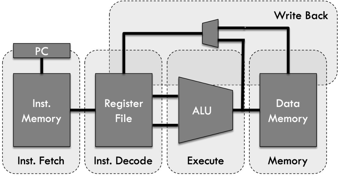
- Stages:
- IF (Instruction Fetch): fetch the instruction from instruction memory
- ID (Instruction Decode): decode the instruction and read the registers
- EX (Execute): perform the arithmetic/logic operation or compute an address
- MEM (Memory Access): access data memory
- WB (Write Back): write the result back to the register
- Pipeline bottleneck: limited by the stage with the longest latency (which determines the clock cycle)
RV32I vs RV64I
- The instruction length is 32 bits in both
- Register width and address space are 32/64 bits
- Standard extensions
- M (multiplication/division)
- A (atomic operations)
- F (single-precision floating point)
- D (double-precision floating point)
- V (vector processing)
RISC-V Instructions
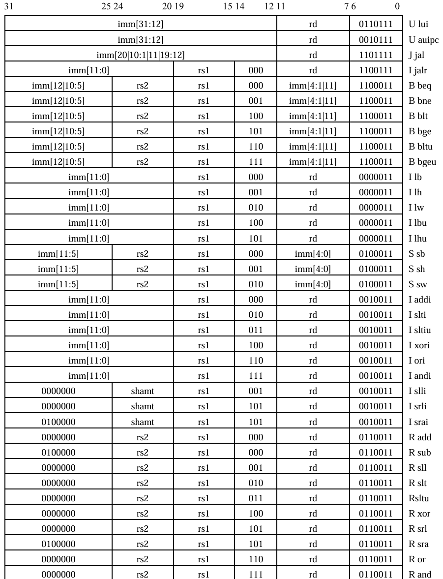
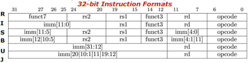
Loading large immediates
lui rd, imm: shift the 20-bit immediate left by 12 bits and store it in rdauipc rd, imm: store PC + (imm << 12) in rd (used for long jumps)
Conditional branches
| beq | bne | blt | bge | bltu(unsigned) | bgeu(unsigned) |
|---|---|---|---|---|---|
| = | != | < | >= | < | >= |
Shift operations
- Left shift:
sll/slli(logical = arithmetic) - Right shift:
srl(logical),sra(arithmetic, fills with the sign bit)
- Left shift:
Sign-extension strategy
lb: load a byte, then sign-extendlbu: load a byte, then zero-extend
Jumps
jal rd, offset: jump to offset; rd stores the return address PC+4jalr rd, rs1, offset: jump to rs1 + offset; rd stores the return address PC+4- jal has a limited jump range, while jalr can jump to any address, which is how the function-return mechanism is implemented
RISC-V Conventions
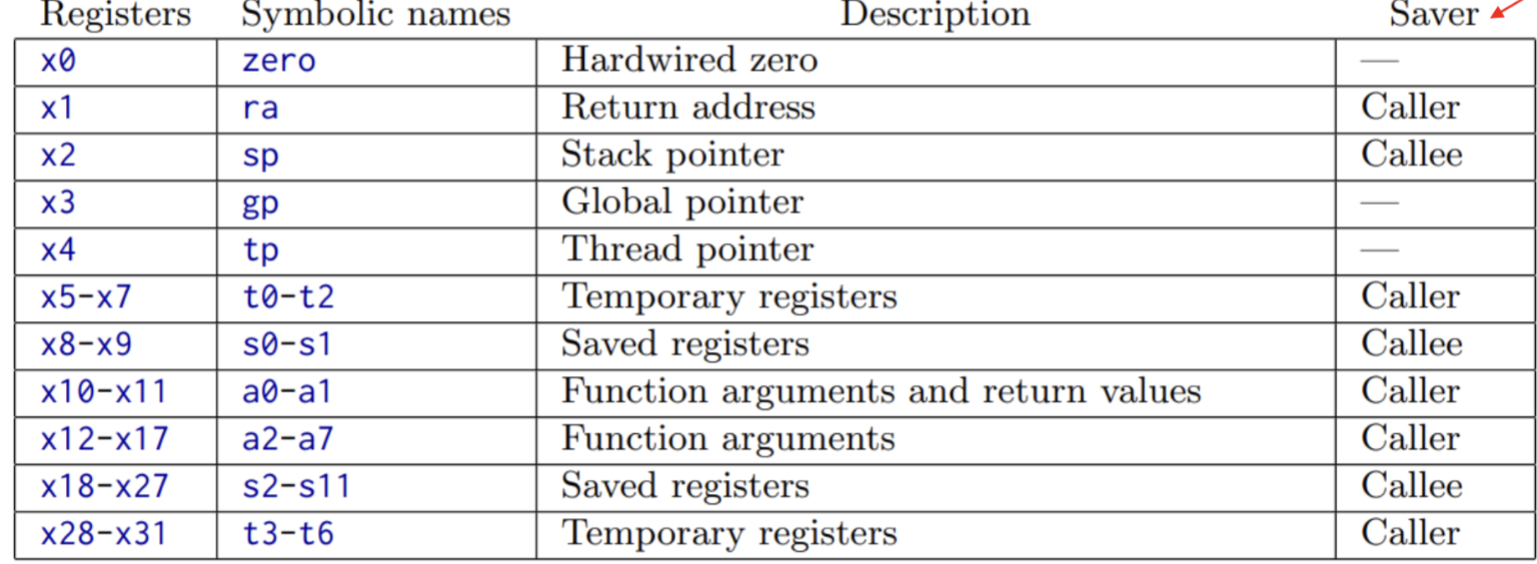
ret: jalr x0, x1, 0 (jump to the address in x1)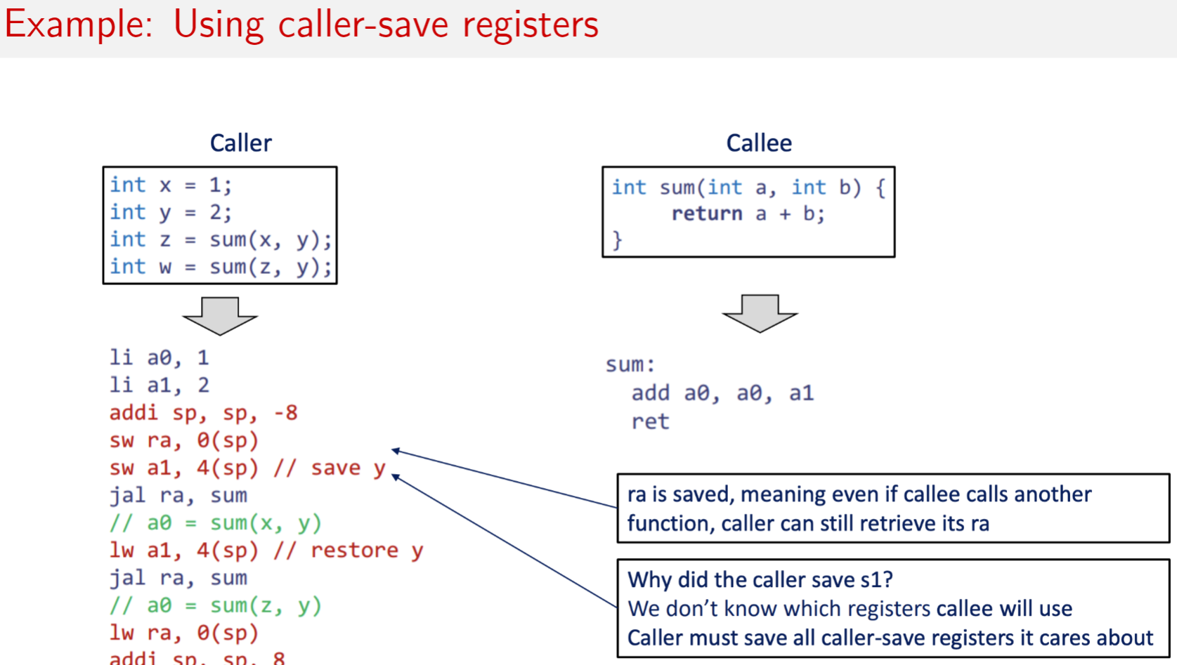
- Before a function call, save all caller-saved registers that the caller uses, and restore them after the function call returns
- Inside a function, when a callee-saved register is used, save it first and restore it afterwards
Processor
Need registers between stages to hold information produced in previous cycle
Hazard
- Structural hazards
- Resource conflicts (e.g., a single-port memory conflict) → separate instruction/data caches
- Data hazards
- Forwarding: route the EX/MEM or MEM/WB result directly to the ALU input (EX stage)
- Condition:
EX/MEM.RegisterRd == ID/EX.RegisterRs
- Condition:
- Load-use hazard: a 1-cycle bubble must be inserted (cannot be solved by forwarding, since the loaded value is only usable after write-back)
- Forwarding: route the EX/MEM or MEM/WB result directly to the ALU input (EX stage)
- Control hazards
- Branch prediction: static (predict not taken by default) vs. dynamic (2-bit predictor + BTB)
- Early branch resolution: compute the target address and condition in the ID stage → fewer bubbles
Instruction reordering: resolves load-use hazards and avoids bubbles
Control Signals
Summary Table of Key Processor Control Signals
| Control signal | Function | Values | Effect on data flow | Typical use case | |
|---|---|---|---|---|---|
| ALUSrc | Selects the source of ALU operand 2 | 0=register file1=immediate | Determines whether the ALU uses a register value or an immediate | addi x1, x2, 100(immediate add) | |
| MemtoReg | Selects the source of the write-back data | 0=ALU result1=memory data | Controls whether the write-back data is the computed result or the value loaded from memory | ld x1, 0(x2)(load instruction) | |
| PCSrc | Selects the source of the next instruction address | 0=PC+41=branch target address | Determines sequential execution or jumping to the branch target | beq x1, x2, label(conditional branch) | |
| RegWrite | Register write enable | 0=write disabled1=write enabled | Controls whether the computed result is written to the register file | All instructions that write a register | |
| ForwardA | Forwarding select for ALU operand 1 | 00=register file10=EX/MEM result01=MEM/WB result | Resolves data hazards in the EX stage by supplying the latest operand | add x1,x2,x3sub x4,x1,x5 | |
| PCWrite | Program counter update control | 0=freeze PC1=update PC | Stalls instruction fetch when a load-use hazard occurs | ld x1,0(x2) followed by add x3,x1,x4 | |
| MemRead | Data memory read enable | 0=read disabled1=read enabled | Controls whether data is read from memory | All load instructions | |
| MemWrite | Data memory write enable | 0=write disabled1=write enabled | Controls whether data is written to memory | All store instructions |
Hazard resolution chain
MemRead→ detect a load-use hazard →PCWrite=0freezes the pipeline →Forwardsupplies the data →RegWritewrites backBranch control flow
WhenPCSrc=1, the default PC update path is overridden → the instructions on the wrong path must be flushed (clear the IF/ID register)Data forwarding
ForwardA: forwarding select for ALU operand 1ForwardB: forwarding select for ALU operand 2
Branch Prediction
Static Branch Prediction
- Predict not taken: assume the branch is not taken
- Target-address based: assume the branch always jumps to a fixed address
Dynamic Branch Prediction
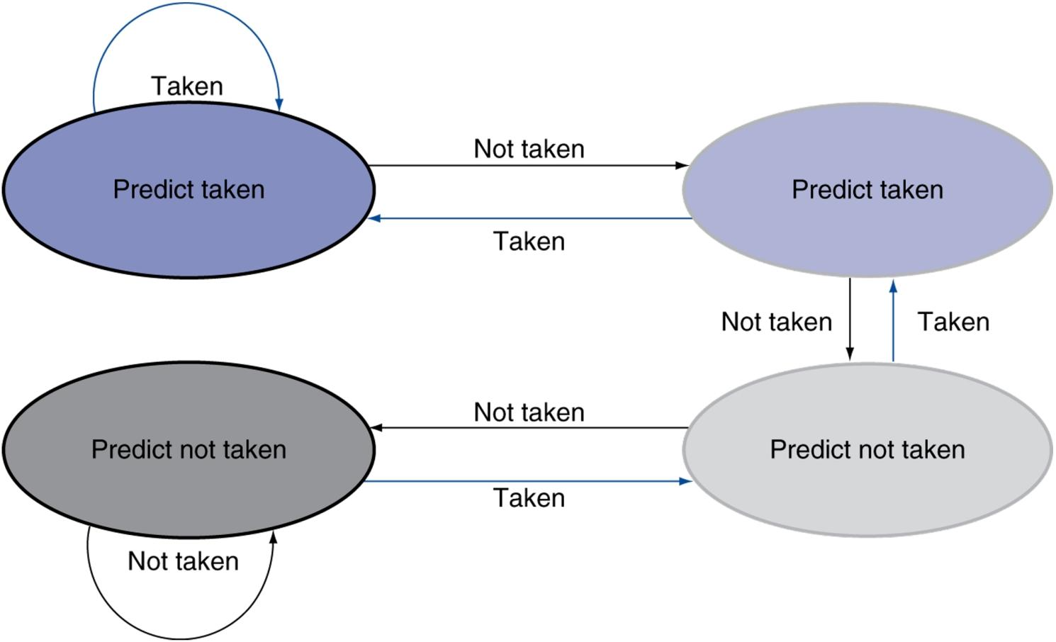
- Two-bit saturating counter: a 2-bit state machine predicts the branch
00: strongly not taken01: weakly not taken10: weakly taken11: strongly taken
- Branch Target Buffer (BTB): stores the target addresses of branch instructions
- Branch history table: records the outcomes of recent branches and updates the prediction state
Handling Mispredictions
- Branch misprediction: detected in the EX stage
- Flush the IF/ID register: if the prediction was wrong, clear the registers of the instruction fetch and decode stages
- Update the PC: set the PC to the correct target address
- Refetch instructions: fetch instructions again from the correct address
Processor Performance
- CPI (Cycles Per Instruction): the average number of clock cycles per instruction = base CPI (ideally 1) + hazard bubbles (data hazards, branch mispredictions)
Memory Hierarchy
Disk Access Time
- Disk access time = seek time + rotational latency + transfer time
- Rotational latency = average rotational latency = 1/2 * (rpm / 60)
Cache
Direct Mapped Cache
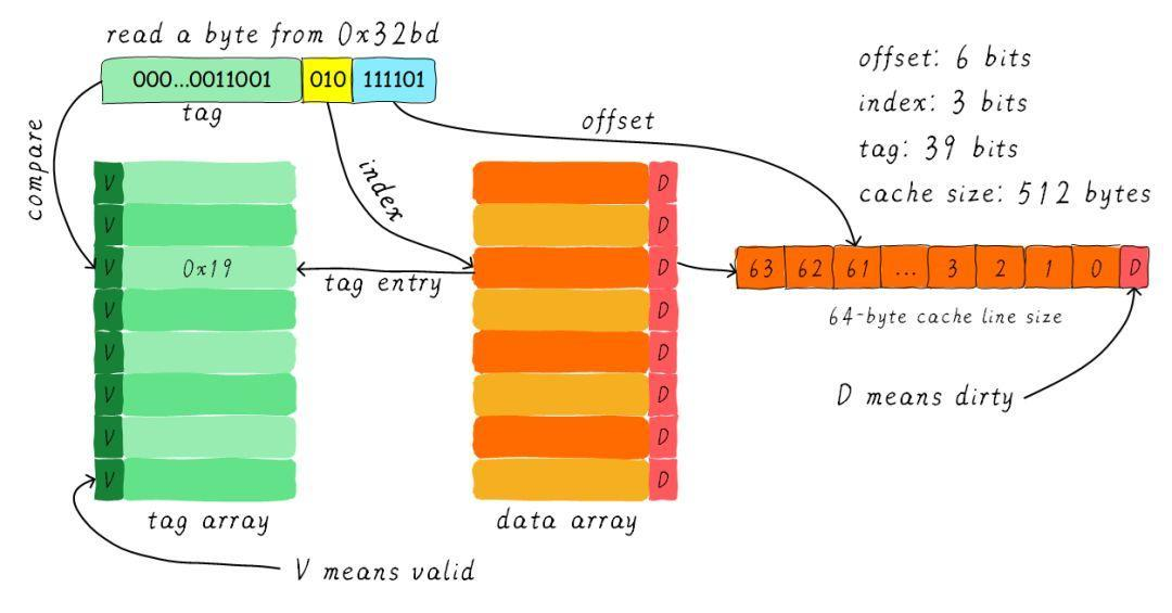
- Unique mapping rule: memory block address
modnumber of cache blocks → determines a unique cache location
Formula:cache index = (block address) % (number of cache blocks) - Address structure:
1
| 高位 Tag 位 | 中位 Index 位 | 低位 Offset 位 |
- Access procedure:
- Use
Indexto locate the cache line - Check the
Validbit - Compare the
Tagbits - If they match and the line is valid → hit; read the data using
Offset
- Use
Set Associative Cache
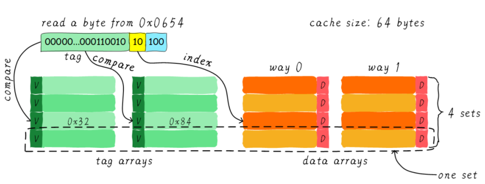
- Set-based mapping:
- The cache is divided into S sets, each containing W ways
- A memory block maps to a specific set, but can be placed in any way within that set
Formula:set index = (block address) % (number of sets S)
- Address structure:
1
| Tag 位 | Set Index 位 | Offset 位 |
- Access procedure:
- Use
Set Indexto locate the set - Compare the W tags in the set in parallel
- Any valid match → hit
- Use
- Multi-way set associative
Replacement Policy (when the set is full)
- LRU (Least Recently Used):
Record access timestamps and replace the block that has gone unused the longest (high hardware cost) - Random replacement:
Randomly pick a way to replace (simple; performance close to LRU)
Fully Associative Cache
- Free mapping: a memory block can be placed in any cache location
- Address structure:
1
| 高位 Tag 位 | 低位 Offset 位 | // 无Index位
- Access procedure:
- Compare the tags of all cache blocks in parallel
- Any valid match → hit
Replacement Policy
- LRU: must be implemented (otherwise performance degrades severely)
- Hardware cost:
Recording the access order of every block is extremely expensive (e.g., a 64KB cache needs 1024 comparators)
Write Policies
- Write hit
- Write-Through: update the cache and memory at the same time (strong consistency, slow).
- Write-Back: update only the cache; write back to memory on eviction (mark the Dirty bit).
- Write miss
- Write-Allocate: load the missing block into the cache, then modify it.
- Write-Around: write directly to memory without loading it into the cache.
Virtual Memory
- Paging: virtual address → physical address (the page size is usually 4KB).
- Page Table:
- Stores the mapping from virtual page numbers to physical page frames / disk addresses.
- A page table entry (PTE) contains Valid, Dirty, and Reference bits.
- Page Fault handling:
When the page is not in memory, load it from disk (takes millions of cycles); handled by the OS.
TLB
- Caches frequently used PTEs to speed up address translation.
- TLB miss handling:
- The hardware loads the PTE (simple page tables) or a software exception handler runs (complex page tables).
Replacement and Write Policies
- LRU replacement: uses the Reference bit to track usage.
- Write-back policy: a Dirty page is written back to disk when it is evicted.
Parallel Processors
Vector Processors
- Core idea: a single instruction operates on a vector register (a group of data elements).
- Advantages:
- Reduced instruction bandwidth (1 instruction performs N operations).
- Sequential memory access patterns, which optimize prefetching and bandwidth utilization.
- RISC-V Vector Extension (RVV):
- 32 vector registers (64 elements per register), supporting instructions such as
vadd.vv(vector add) andfmul.d.vs(scalar times vector).
- 32 vector registers (64 elements per register), supporting instructions such as
- Key optimizations:
- Chaining: element-level pipeline forwarding, which resolves RAW hazards.
- Multi-lane: process multiple elements in parallel to increase throughput.
- Masking: conditional execution (e.g.,
fcmp.neq.v+fsub.vimplements a conditional subtraction).
SIMD extensions (e.g., Intel AVX)
- Wide registers integrated into the CPU (e.g., 512-bit AVX, supporting 16 single-precision floating-point operations in parallel).
- Use cases: dense computation (image processing, scientific computing).
GPU
Core architecture (NVIDIA Fermi as an example)
- Streaming Multiprocessor (SM):
- 32 CUDA cores (each supporting floating-point/integer operations).
- 16 load/store units + 4 special function units (sin/exp, etc.).
- 32K register file + 64KB shared memory/L1 cache.
- SIMT execution model:
- Threads are scheduled in warps of 32 threads.
- Hardware multithreading switches hide memory latency.
- Streaming Multiprocessor (SM):
CPU vs. GPU design philosophy
| Component | CPU | GPU |
|————————|————————————|———————————-|
| Core goal | Low latency, complex control flow | High throughput, data parallelism |
| Cache | Large multi-level caches | Small caches; relies on high-bandwidth graphics memory|
| Transistor allocation | Control logic, branch prediction | Floating-point units, multithreading contexts|
| Use cases | Serial code, task scheduling | Parallel computation (AI/HPC) |
Domain Specific Architectures
Inefficiency of General-Purpose Architectures (Turing Tariff)
- Problem: general-purpose processors (CPU/GPU) are inefficient when executing specific tasks, incurring performance and energy overhead.
- Reason: control overhead such as instruction fetch, decode, and branch prediction consumes a large share of the energy (90%–99.9%).
- Data comparison:
- 32-bit integer add (28nm process): an ASIC needs only 68fJ, while an ARM A15 CPU needs 250pJ (about 4000x the energy).
- Solutions:
- Hardware-centric: DSAs (domain-specific architectures) optimized for a specific domain.
- Software-centric: domain-specific languages (DSLs) such as TensorFlow/PyTorch, which express operator structure explicitly.
- Hybrid approach: DSA + DSL combinations (e.g., TPU + TensorFlow).
Sources of DSA Speedup
- Four main optimization techniques:
- Data specialization
- Custom data types (e.g., 4-bit compressed weights) to reduce memory footprint (e.g., the EIE accelerator cuts memory usage by 30x).
- Parallelism
- Massively parallel units (e.g., the TPU’s systolic array); memory bottlenecks must be avoided.
- Locally optimized memory
- Small SRAM replaces DRAM: an SRAM read costs 5pJ/bit versus 640pJ/bit for a DRAM read (a 128x difference).
- Data compression increases effective bandwidth (e.g., weight sparsification in NVDLA increases on-chip memory capacity by 3–10x).
- Overhead reduction
- Eliminate control overhead such as instruction fetch/decode and branch prediction.
- Low-precision computation (e.g., 8-bit integers instead of 32-bit floating point).
- Data specialization
DSAs in AI Acceleration
- Core operators: matrix multiplication (GEMM) and convolution (Conv) account for more than 90% of DNN computation (e.g., AlexNet).
- Memory bottleneck optimization:
- Data reuse:
- Convolutional reuse (sliding window), feature-map reuse (batching), filter reuse.
- Data reuse:
DSAs in the RISC-V Ecosystem
- Customization flow:
- Extend the instruction set: add RoCC (Rocket Chip Coprocessor) custom instructions.
- Integrate the accelerator: connect it to the RISC-V core through a decoupled interface (Ready-Valid protocol).
- Development tools: use the Chipyard platform to generate RTL, with support for FPGA simulation and ASIC tape-out.
- RoCC mechanism:
- Instruction format: inherits the RISC-V R-type; the
xd/xs1/xs2flags control data transfer. - Communication interfaces:
- Command interface: sends the instruction +
rs1/rs2data to the accelerator. - Response interface: the accelerator writes the result back to the
rdregister.
- Command interface: sends the instruction +
- Advantage: supports DMA direct memory access, avoiding the cache-coherence bottleneck.
- Instruction format: inherits the RISC-V R-type; the
Selected Readings from CAAQA
The implementation of a computer covers two aspects: organization and hardware
1.9 Quantitative Principles of Computer Design
1.9.1 Take Advantage of Parallelism
- System-level parallelism: use multiple processors/storage devices
- Processor-level parallelism: use multicore processors / instruction-level parallelism (pipelining, superscalar)
- Digital-design-level parallelism: use parallel circuits such as multiplexers and adders
1.9.2 Principle of Locality
Programs tend to reuse the data and instructions they have used recently
- Temporal locality
- Spatial locality
1.9.4 Amdahl’s Law
- The performance improvement of a computer system is limited by its slowest part
- Speedup =
- p: the fraction that is sped up
- s: the speedup factor
1.9.5 The Processor Performance Equation
- CPU time = CPU clock cycles * clock cycle time
- CPI (clock cycles per instruction) = CPU clock cycles / instruction count
- Processor performance = clock frequency instructions per clock cycle (CPI) instruction count
2.4 Virtual Memory
Divide physical memory into blocks and assign them to different processes
Translated from the Chinese original.