A comprehensive algorithms review, summarizing the key topics: divide and conquer, graph algorithms, dynamic programming, linear programming, P vs NP, reductions, and more.

Divide and Conquer

Master theorem:

for some constants (a>0) , (b>1) ,and (d ≥0) , then

d is the exponent of the time complexity of the non-recursive part (i.e., the work done outside each recursive call).

Proof: analyze the total work in the recursion tree

FFT

Graph Algorithms

DFS

1
2
3
4
5
6
7
8
9
10
11
12
13
14

EXPLORE(G, v):  
1. visited[v] = true  
2. pre[v] = clock; clock++      # 记录发现时间  
3. for each edge (v, u) ∈ E:  
4.    if not visited[u]:  
5.        EXPLORE(G, u)  
6. post[v] = clock; clock++     # 记录离开时间  

DFS(G):  
1. for all v ∈ V: visited[v] = false  
2. clock = 0  
3. for all v ∈ V:  
4.    if not visited[v]:  
5.        EXPLORE(G, v)  

running time: O(|V|+|E|)

SCC (Strongly Connected Components)

1
2
3
4
5
6
7
8
9
10
11
12
13

Input: 有向图 G = (V, E)
Output: G 的强连通分量
1. DFS(G)  # 执行 DFS，记录每个节点的 post 时间
2. 按 post 时间降序排列 V
3. G' = G 的转置图 （将所有边反向）
4. visited = false for all v ∈ V
5. for each v in V (按 post 时间降序):
6.    if not visited[v]:
7.        SCC = {}  # 当前强连通分量
8.        EXPLORE(G', v)  # 在转置图上进行 DFS
9.        for each u in SCC:
10.           visited[u] = true  # 标记已访问
11.           print(u)  # 输出当前强连通分量的节点

running time: O(|V|+|E|)

Dijkstra

1
2
3
4
5
6
7
8
9
10
11
12
13
14

**Input**: 图 G, 边权 ℓ, 起点 s  
**Output**: 所有节点到 s 的最短距离 dist[]  

1. for each u ∈ V:  
2.    dist[u] = ∞; prev[u] = nil  
3. dist[s] = 0  
4. H = 优先队列 (key=dist)   # 初始包含所有节点  
5. while H 非空:  
6.    u = H.deletemin()     # 取出 dist 最小的节点  
7.    for each 边 (u, v) ∈ E:  
8.        if dist[v] > dist[u] + ℓ(u, v):  
9.            dist[v] = dist[u] + ℓ(u, v)  
10.           prev[v] = u  
11.           H.decreasekey(v)  # 更新 v 在队列中的优先级  

Bellman-Ford

1
2
3
4
5
6
7
8
9
10
11
12
13
14

**Input**: 图 G, 边权 ℓ, 起点 s（无负环）  
**Output**: 最短距离 dist[]，或报告负环  

1. for each u ∈ V:  
2.    dist[u] = ∞; prev[u] = nil  
3. dist[s] = 0  
4. repeat |V| - 1 次:  
5.    for each 边 e = (u, v) ∈ E:  
6.        if dist[v] > dist[u] + ℓ(u, v):  
7.            dist[v] = dist[u] + ℓ(u, v)  
8.            prev[v] = u  
9. for each 边 e = (u, v) ∈ E:  
10.   if dist[v] > dist[u] + ℓ(u, v):  
11.       return "存在负环"  

running time: O(|V| * |E|)

Shortest Paths in a DAG

A topological order is a linear ordering of the vertices of a directed acyclic graph (DAG) in which, for every edge (u, v), u comes before v.

1
2
3
4
5
6
7
8
9
10
11
12

Input: DAG G, 边权 ℓ, 起点 s  
Output: 最短距离 dist[]  

1. for each u ∈ V:  
2.    dist[u] = ∞; prev[u] = nil  
3. dist[s] = 0  
4. L = 拓扑排序(G)   # 按线性序排列节点  
5. for each u ∈ L (按序处理):  
6.    for each 边 (u, v) ∈ E:  
7.        if dist[v] > dist[u] + ℓ(u, v):  
8.            dist[v] = dist[u] + ℓ(u, v)  
9.            prev[v] = u  

running time: O(|V| + |E|)

MST (Minimum Spanning Tree)

1
2
3
4
5
6
7
8
9
10
11
12
13
14
15
16
17
18
19
20
21
22
23

Kruskal(G)
// Input: 无向图 G = (V, E)
// Output: 最小生成树 T
1. T = ∅  // 初始化最小生成树
2. for each edge (u, v) ∈ E in increasing order of weight:
3.    if u and v are in different components:
4.        T = T ∪ {(u, v)}  // 添加边到最小生成树
5.        union(u, v)  // 合并 u 和 v 的连通分量

Prim(G, s)
// Input: 无向图 G = (V, E), 起点 s
// Output: 最小生成树 T
1. T = ∅  // 初始化最小生成树
2. for each vertex v ∈ V: dist[v] = ∞; prev[v] = nil
3. dist[s] = 0  // 起点到自身的距离为 0
4. H = 优先队列 (key=dist)  // 初始化优先队列
5. while H 非空:
6.    u = H.deletemin()  // 取出距离最小的节点
7.    for each 边 (u, v) ∈ E:
8.        if dist[v] > ℓ(u, v):  // 如果找到更小的边
9.            dist[v] = ℓ(u, v)  // 更新距离
10.           prev[v] = u  // 更新前驱节点
11.           H.decreasekey(v)  // 更新优先队列中的优先级

Cut property: for any cut (S, V-S) of a graph G, the minimum-weight edge crossing between S and V-S must belong to some MST.

1
2
3
4
5
6
7
8
9
10
11
12
13
14
15
16
17
18
19
20
21
22
23

并查集

# 初始化单元素集合  
makeset(x):  
1. π[x] = x      # 父指针  
2. rank[x] = 0   # 秩  

# 查找根（带路径压缩）  
find(x):  
1. if x ≠ π[x]:  
2.   π[x] = find(π[x])  # 递归压缩路径  
3. return π[x]  

# 合并集合（按秩合并）  
union(x,y):  
1. rx = find(x), ry = find(y)  
2. if rx == ry: return  
3. if rank[rx] > rank[ry]:  
4.   π[ry] = rx  
5. else:  
6.   π[rx] = ry  
7.   if rank[rx] == rank[ry]:  
8.     rank[ry]++  

Dynamic Programming

Dynamic Programming

• Core idea: break the problem into overlapping subproblems and store the subproblem solutions to avoid redundant computation.
• Key steps:
  1. Define the subproblems
  2. Set up the recurrence (state transition equation)
  3. Determine the evaluation order (bottom-up or memoized search)
• Applications:
  • Longest Increasing Subsequence (LIS): length of the LIS ending at j $L(j) = 1 + \max\{L(i) \mid i < j, a_i < a_j\}$
  • Edit distance: the minimum cost of aligning two strings, $E(i,j) = \min\{1+E(i-1,j), 1+E(i,j-1), \text{diff}(i,j)+E(i-1,j-1)\}$
  • Knapsack:
    • Knapsack with repetition: $K(w) = \max_{i} \{K(w - w_i) + v_i\}$
    • 0/1 knapsack: $K(w,j) = \max \{K(w-w_j, j-1) + v_j, K(w, j-1)\}$
  • Matrix chain multiplication: minimize the number of multiplications, $C(i,j) = \min_{k} \{C(i,k) + C(k+1,j) + m_{i-1}m_k m_j\}$
  • Traveling Salesman Problem (TSP): C(S,j) is the shortest path that passes through the set S and ends at j; complexity O(n^2 2^n).
  • Independent set on a tree: maximum independent set size $l(u) = \max \{1 + \sum \text{grandchildren } l(w), \sum \text{children } l(w) \}$

LIS (Longest Increasing Subsequence)

1
2
3
4
5
6
7
8
9

Input: 序列 a[1..n]  
Output: LIS 长度  

1. for j = 1 to n:  
2.   L[j] = 1  # 初始化以 j 结尾的 LIS 长度  
3.   for i = 1 to j-1:  
4.     if a[i] < a[j]:  
5.       L[j] = max(L[j], L[i] + 1)  
6. return max(L)  

running time: O(n^2)

LCS (Longest Common Subsequence)

1
2
3
4
5
6
7
8
9
10
11

Input: 序列 a[1..n], b[1..m]
Output: LCS 长度
1. for i = 0 to n: L[i,0] = 0  # 初始化第一行
2. for j = 0 to m: L[0,j] = 0  # 初始化第一列
3. for i = 1 to n:
4.   for j = 1 to m:
5.     if a[i] == b[j]:
6.       L[i,j] = L[i-1,j-1] + 1  # 匹配时长度加1
7.     else:
8.       L[i,j] = max(L[i-1,j], L[i,j-1])  # 不匹配时取最大
9. return L[n,m]  # 返回 LCS 长度

running time: O(n*m)

0/1 Knapsack

1
2
3
4
5
6
7
8
9
10
11

Input: 物品重量 w[1..n], 价值 v[1..n], 容量 W  
Output: 最大价值  

1. for w = 0 to W: K[w,0] = 0  
2. for j = 1 to n:  
3.   for w = 1 to W:  
4.     if w_j > w:  
5.       K[w,j] = K[w,j-1]  
6.     else:  
7.       K[w,j] = max(K[w-w_j,j-1] + v_j, K[w,j-1])  
8. return K[W,n]  

Linear Programming

MAX Flow

1
2
3
4
5
6
7
8
9
10
11

FORD-FULKERSON(G, s, t):
    for each edge (u,v) in G:
        f(u,v) = 0  // 初始化流量
    while exists path p from s to t in residual graph G_f:
        c_f(p) = min{ c_f(u,v) | (u,v) in p }  // 路径剩余容量
        for each edge (u,v) in p:
            if (u,v) is forward edge:
                f(u,v) += c_f(p)
            else:  // (v,u)是反向边
                f(v,u) -= c_f(p)  // 减少正向流量
    return f  // 最大流

The idea behind Ford-Fulkerson:

• Build the residual graph: residual capacity of a forward edge = c_e - f_e, capacity of a backward edge = f_e
• Iteratively search for augmenting paths: use BFS/DFS to find an s→t path in the residual graph
• Update the flow: push an amount equal to the minimum residual capacity along the path
• Complexity: O(|V|·|E|²)

Max Flow-Min Cut theorem: the maximum flow equals the minimum cut, i.e., in a flow network, the maximum flow from the source to the sink equals the minimum total capacity of the edges cut when the network is split into two parts.

Bipartite matching can be solved by reducing it to max flow: turn the bipartite graph into a flow network, connect the source to the left-side vertices, connect the right-side vertices to the sink, and give every edge capacity 1.

Simplex

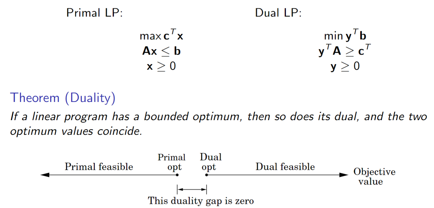
Dual LP

P vs NP

Class P:

• Decision problems that can be solved by a polynomial-time algorithm
• Time complexity O(n^k), where k is a constant

Class NP:

• Decision problems for which, given a solution, its correctness can be verified in polynomial time
• Nondeterministic Polynomial time

NP-Complete problems:

• Problems that belong to NP
• Every problem in NP can be reduced to them in polynomial time
• If any NP-Complete problem has a polynomial-time algorithm, then P = NP

NP-Complete

Search Problem: given an instance I and a solution checker C(I,S) (polynomial-time verification), find a solution S

Search problems are equivalent to NP problems.

Reductions

A -> B (A is no harder than B, A <= B)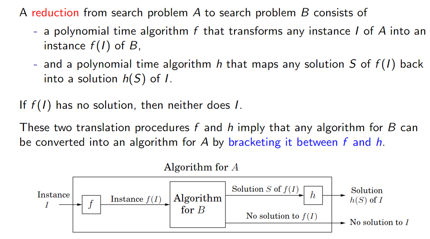

Key points:

• Instance transformation
• Solution transformation (including passing along “no solution”)
• Both done in polynomial time

For non-search problems, only the instance transformation is needed.

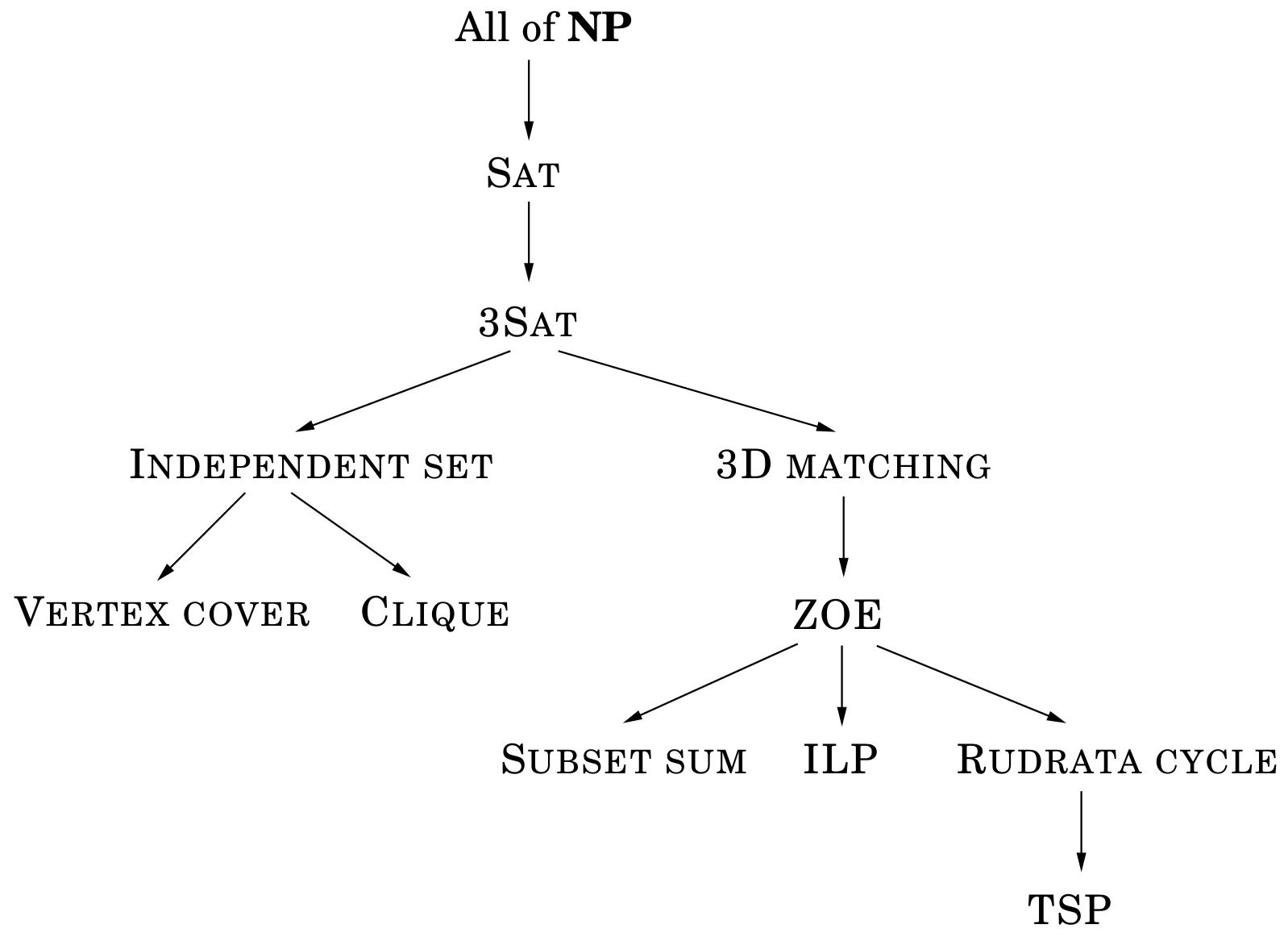
Reduction chain analysis: 3SAT → INDEPENDENT SET → VERTEX COVER → CLIQUE

1. 3SAT → INDEPENDENT SET

• Goal: reduce Boolean satisfiability (3SAT) to the independent set problem.

• Steps:
  a. Instance transformation:

  • For a 3SAT formula with k clauses, construct a graph G:
    • Each clause becomes a triangle (3 vertices), whose vertices represent the literals in the clause (e.g. $x, \neg y$).
    • Add conflict edges: if two literals are complementary (e.g. x and ), connect them across all triangles.
  • Set the target independent set size g = k (the number of clauses).
    Example: the formula $(x \lor y \lor z) \land (\neg x \lor \neg y)$
    → two triangles: ${x,y,z} \text{ and } {\neg x, \neg y, \text{dummy}}$, and add the edges $(x, \neg x), (y, \neg y)$

  b. Solution transformation:

  • If an independent set of size g exists, then exactly one vertex is chosen from each triangle (the conflict edges guarantee that complementary literals are never both chosen).
  • Set the chosen literals to true (e.g. if x is chosen then x=true; if is chosen then x=false

• Key insight:
  Choosing the independent set = picking one true literal per clause, with a globally consistent assignment.

2. INDEPENDENT SET → VERTEX COVER

• Goal: reduce independent set to the vertex cover problem.

• Steps:
  a. Instance transformation:

  • Given a graph G=(V,E) and independent set target g, use the very same graph G
  • Set the vertex cover target b = |V| - g (e.g. |V|=5, g=2 → b=3

  b. Solution transformation:

  • If a vertex cover C of size b exists, then $V \setminus C$ is an independent set of size g.
    (because C covers every edge → there are no edges inside $V \setminus C$)
  • If an independent set S of size g exists, then $V \setminus S$ is a vertex cover of size b.

• Key insight:
  Independent set and vertex cover are complementary problems: $$S \text{ is an independent set} \iff V \setminus S \text{ is a vertex cover}$$

3. VERTEX COVER → CLIQUE

• Goal: reduce vertex cover to the clique problem.

• Steps:
  a. Instance transformation:

  • Given a graph G=(V,E) and vertex cover target b, construct its complement graph
  • Set the clique target g = |V| - b (e.g. |V|=4, b=1 → g=3

  b. Solution transformation:

  • If has a clique K of size g, then $V \setminus K$ is a vertex cover of G of size b.
    (since K is a complete subgraph in → it has no edges in G → covers every edge of G)
  • If G has a vertex cover C of size b, then is a clique of size g in .

  c. Passing along “no solution”:

  • If has no clique of size g, then G has no vertex cover of size b.

• Key insight:
  The complement of a vertex cover is a clique in the complement graph:

  $$C \text{ is a vertex cover} \iff V \setminus C \text{ is a clique in } \bar{G}$$

Other Algorithms

Euclid’s Algorithm

1
2
3
4
5
6
7
8
9
10
11
12

Euclid(a, b) 
// Input: two integers a and b with a ≥b ≥0
// Output: gcd(a, b)
1. if b = 0 then return a
2. return Euclid(b, a mod b)

extended-Euclid (a, b) 
// Input: two integers a and b with a ≥b ≥0
// Output: gcd(a, b) and integers x and y such that ax + by = gcd(a, b)
1. if b = 0 then return (a, 1, 0)
2. (g, x1, y1) = extended-Euclid(b, a mod b)
3. return (g, y1, x1 - (a / b) * y1)

For any positive integers a and b ,the extended Euclid algorithm returns integers x , y ,and d such that go $d(a, b)=d=a x+b y$

RSA

1
2
3
4
5
6
7
8
9
10
11
12

1. 随机选择大素数 p, q → 计算 N = p * q
2. 选 e 满足 gcd(e, (p-1)(q-1)) = 1 （互素）
3. 计算 d = e⁻¹ mod (p-1)(q-1)  // 扩展欧几里得（ed ≡ 1 mod φ(n)）
4. 公钥 = (N, e), 私钥 = d

RSA(n, e, m)
// Input: n = p * q, e, m（明文）
// Output: c = m^e mod n

RSA-decrypt(n, d, c)
// Input: n = p * q, d, c
// Output: m = c^d mod n

The correctness of RSA rests on Euler’s theorem:

If gcd(m, n) = 1, then m^φ(n) ≡ 1 (mod n)

Prime Testing

Fermat’s little theorem: if p is prime and a is any integer, then a^(p-1) ≡ 1 (mod p)

1
2
3
4
5
6
7

primality2(N) 
// Input: positive integer N 
// Output: yes/no 
1. Pick positive integers a1, a2, ..., ak<N at random 
2. if ai^{N-1} ≡ 1 (mod N ) for all i=1,2, ..., k 
then return yes 
3. else return no. 

Pr(primality2 returns yes when N is not prime) ≤ 1 / 2^k

Translated from the Chinese original.