CS2314: lecture notes for Intelligent Speech Technology, taught by Professors Yanmin Qian and Kai Yu.

Lec1

Fourier Transform

Formula:

Properties of the Fourier transform:

• Linearity:
• Time shift:
• Frequency shift:

Spectral Properties of Periodic and Aperiodic Signals:

• The spectrum of a periodic signal is discrete; every frequency component in the spectrum is an integer multiple of the fundamental frequency

• The spectrum of an aperiodic signal is continuous.

• The spectrum of a periodic signal is discrete, with spectral-line spacing

• The amplitude varies as $Sa( \frac{nπτ}{T_{1}})$ or . When , the envelope of the spectral lines crosses zero

• A periodic signal contains infinitely many spectral lines, but according to its envelope the energy is mainly concentrated
  within the first zero crossing (0 ∼ ), i.e. the low-frequency part of the signal carries most of the energy.

The Sampling Function

The shape of the spectral envelope of a periodic rectangular pulse train depends on the width and the period of the rectangular pulse. When the rectangular pulse has width τ and period T, the envelope of its spectrum takes the shape of the sampling function (the Sa function).
In the spectrum of a periodic rectangular pulse train,

​

The Sampling Theorem

The Nyquist sampling rate is the minimum sampling frequency required so that the sampled discrete signal can exactly reconstruct the original continuous signal; it must be at least twice the highest frequency of the original continuous signal. If the highest frequency of the original signal is $f_{max}$, then the Nyquist sampling rate $f_s$ is given by $f_s \geq 2f_{max}$.

The Convolution Theorem

Time-domain convolution theorem:

Frequency-domain convolution theorem:

Lec2

Laplace Transform

To overcome the limitations of the Fourier transform (which requires the Dirichlet condition of absolute integrability), the Laplace transform decomposes the signal into real and imaginary parts, so that it can handle aperiodic signals.

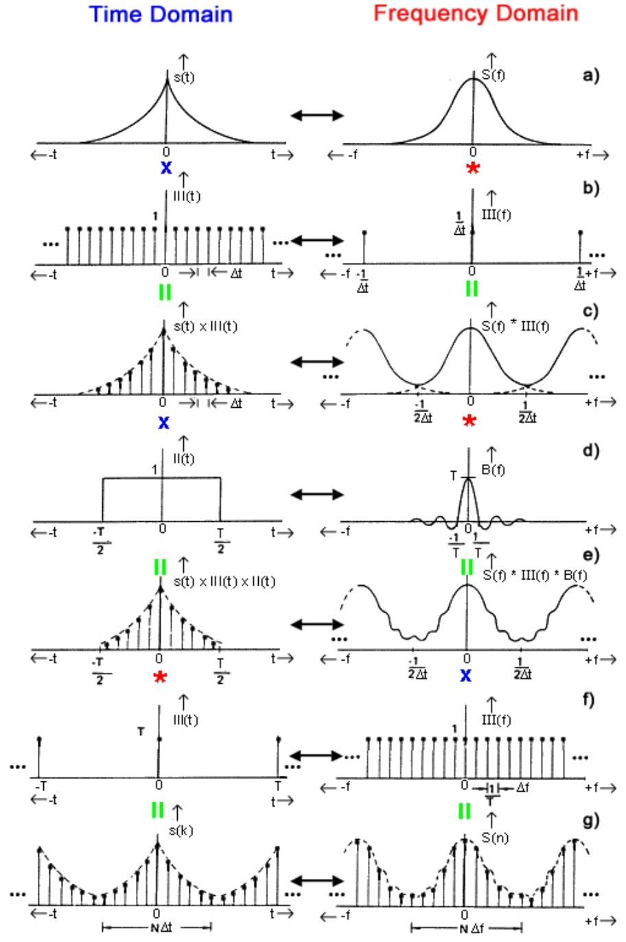
DTFT: Discrete-Time Fourier Transform

Discrete in the time domain, periodic in the frequency domain.

DFT: Discrete Fourier Transform

• Symmetry
  

After taking the DFT of a discrete signal of length N, the magnitude of the k-th frequency component equals the magnitude of the -th frequency component; at the same time, their phases are equal in magnitude but opposite in sign.

• Energy conservation (Parseval’s theorem) $$\sum_{n=0}^{N-1}|x(n)|^{2}=\frac{1}{N} \sum_{n=0}^{N-1}|F[k]|^{2}$$

Window Functions

Framing: overlapping frames are used to represent the dynamic characteristics of speech.

• Rectangular window
• Hann window
• Hamming window
• Blackman window
• Kaiser window
  Choice: the main-lobe width affects frequency resolution, and the side-lobe attenuation affects spectral leakage.

Lec3

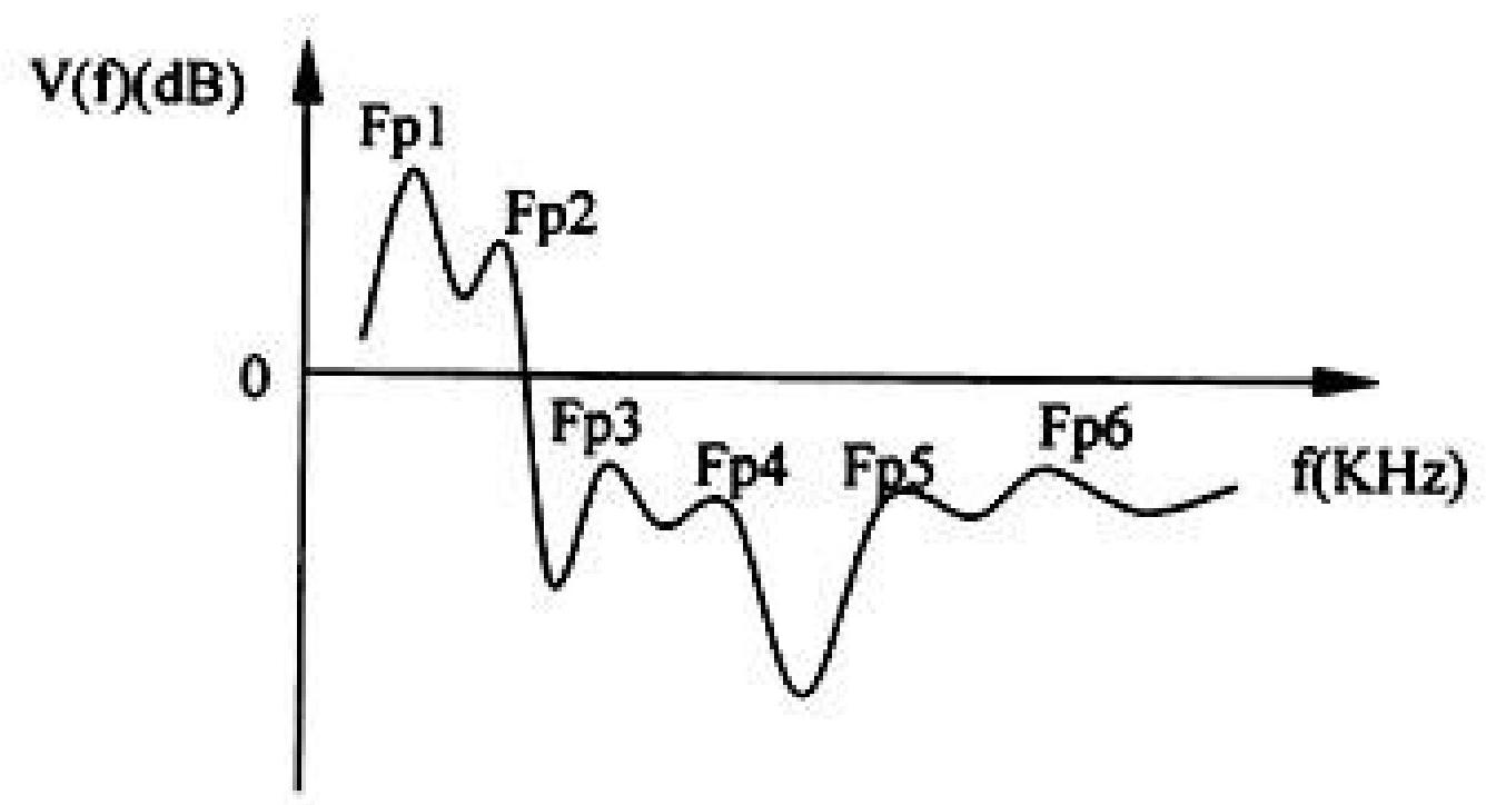
Spectral Features of Voiced Sounds

Formant structure:

Pitch Detection

Pitch detection is a key step in speech signal processing. Its goal is to obtain the periodicity of vocal-fold vibration, providing a foundation for tasks such as speech analysis, synthesis and recognition. There are several pitch detection methods in both the time domain and the frequency domain, each with its own characteristics:

• Time-domain pitch detection methods

  • AMDF method: define the average magnitude difference function $\gamma(l)=\sum{n = 0}^{N - l - 1}\left|S{w}(n + l)-S{w}(n)\right|S{w}(n)l = nTn = 1, 2,\cdotsT\gamma(l)$ approaches a local minimum. This method uses only simple additions and subtractions, which made it suitable for early general-purpose CPUs, on which multiplication was slow. However, in low-SNR environments its robustness to interference is weak and the detection accuracy may suffer.
  • Autocorrelation method: detect the pitch period by defining the autocorrelation function of speech $R(l)=\sum{n = 0}^{N - l - 1} S{w}(n + l) S_{w}(n)l = nTn = 1, 2,\cdotsR(l)$ approaches a local maximum. Digital signal processors have dedicated hardware instructions that perform multiply-accumulate operations quickly, so this method is widely used on DSPs. However, the computational load is relatively large, which places some demands on the hardware’s computing capability.
  • Center-clipping method: first apply center clipping to the speech signal, then compute the autocorrelation function. Exploiting the fact that the local peaks of the autocorrelation function coincide with the amplitude peaks of the speech, the autocorrelation function is computed only at the peak positions, and the pitch period of the signal is then obtained by searching and comparing. This method improves computational efficiency and reduces interference, but center clipping may lose some of the fine detail in the speech signal.
• Frequency-domain pitch detection methods: mainly harmonic analysis, which computes the pitch period by analyzing the spectral-line structure of the voiced signal. Since a voiced signal has a spectral-line structure corresponding to the pitch and its harmonics, the pitch period can be determined by analyzing the relationships between these lines, such as their frequency spacing. This method analyzes the frequency components of the signal fairly accurately and makes effective use of frequency-domain information. However, the frequency-domain transform is computationally expensive and requires the signal to be reasonably stationary; if the speech signal contains abrupt changes or is non-stationary, the detection accuracy may drop.

The Auditory System

1. Auditory Perception Characteristics

1. Loudness Perception

• Relationship between sound pressure level (SPL) and loudness: ( L = k \log(P/P_0) )
• Applications: dynamic range compression of audio signals, loudness equalization

1
2
3
4

def normalize_loudness(signal: np.ndarray) -> np.ndarray:
    # 基于对数关系的响度归一化
    normalized = k * np.log10(np.abs(signal) / reference_pressure)
    return normalized

1. Frequency Resolution [Critical Band]

• Critical bandwidth: narrow at low frequencies (~100Hz), wide at high frequencies (~500Hz)
• Applications: the Mel frequency scale, used for extracting MFCC features

  1 2 3

  def hz2mel(freq: float) -> float: # Hz转Mel频率 return 2595 * np.log10(1 + freq/700)

2. Applications of the Masking Effect

1. Temporal Masking

• Forward masking: ~20ms
• Backward masking: ~200ms
• Applications: audio coding and compression, noise suppression

1. Frequency Masking

• Simultaneous masking: a strong signal masks weaker signals at nearby frequencies
• Applications: audio feature enhancement, speech enhancement

  1 2 3 4 5 6

  def apply_frequency_masking(spectrum: np.ndarray) -> np.ndarray: # 计算掩蔽阈值 masking_threshold = compute_masking_curve(spectrum) # 低于阈值的频率分量被抑制 enhanced = np.maximum(spectrum - masking_threshold, 0) return enhanced

3. Key Points for Engineering Applications

1. Speech feature extraction

• MFCC features: mimic the frequency response of the human ear
• PLP features: incorporate equal-loudness curves
• Gammatone filter bank: mimics the response of the basilar membrane

1. Audio coding optimization

• Bit allocation based on masking thresholds
• Dynamic range compression
• Acoustic echo cancellation

Key conclusions:

• Speech processing systems should focus on the 2kHz-5kHz band (the region where the human ear is most sensitive)
• The nonlinearity of the critical bandwidth inspired the design of the Mel scale
• The masking effect can be used for audio compression and noise reduction

These auditory characteristics provide an important theoretical foundation and optimization directions for speech signal processing.

Lec5

The Gaussian Distribution

1. Expression: a Gaussian distribution with mean and variance is written as $$p(x) \equiv \mathcal{N}\left(\mu, \sigma^{2}\right)=\frac{1}{\sqrt{2\pi\sigma^{2}}}\exp\left\{-\frac{(x-\mu)^{2}}{2\sigma^{2}}\right\}$$

The mean determines the center of the distribution, and the variance determines how spread out it is. The larger the variance, the more dispersed the data and the “shorter and fatter” the curve; the smaller the variance, the more concentrated the data and the “taller and thinner” the curve.

1. Multivariate Gaussian distribution
   • Form: the d-dimensional multivariate Gaussian distribution has the form $p(x)=\frac{1}{(2 \pi)^{\frac{d}{2}}|\sum|^{\frac{1}{2}}} \exp \left\{-\frac{1}{2}(x-\mu)^{\top} \sum^{-1}(x-\mu)\right\}$. When the covariance matrix is diagonal, the expression simplifies to $p(x)=\prod_{i=1}^{d} \frac{1}{\sqrt{2 \pi \sigma_{i}^{2}}} \exp \left\{-\frac{\left(x_{i}-\mu_{i}\right)^{2}}{2 \sigma_{i}^{2}}\right\}$
   • Properties: taking the 2-dimensional Gaussian as an example, the conditional marginal of a Gaussian, the marginal distribution of each component, and the joint marginal distribution of any subset are all Gaussian; if follows a Gaussian distribution and , then is a Gaussian with mean $A\mu{x} + bA\sum{x}A^{\top}$.
2. Expectation and variance: for a multivariate Gaussian , integration gives its expectation , , and covariance .
3. For the Gaussian distribution, independence is equivalent to being uncorrelated

Lec8

Front-end Processing: Voice Activity Detection (VAD)

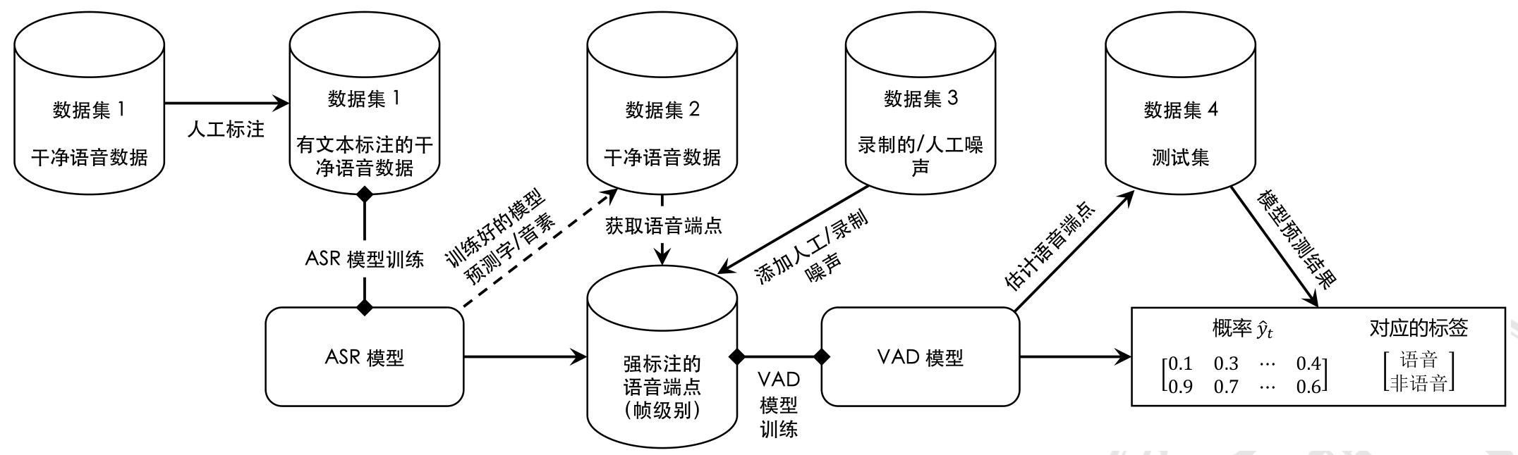
The traditional training pipeline for a supervised VAD model
▶ 1. Collect clean single-speaker speech data, especially data
whose audio quality does not vary much. Make sure the data contains only one or more fixed languages.
▶ 2. Manually transcribe this data.
▶ 3. Train an ASR model on this data.
▶ 4. Use the trained ASR model to predict whether speech is present
in the audio of a new (usually clean) dataset, to obtain frame-level strong labels.
▶ The ASR model can provide phone-level alignments, which are then converted into a binary speech
indicator (frames containing speech are set to 1, silent segments to 0)
▶ 5. Train a VAD model (DNN/CNN/RNN, etc.) on the new dataset using the strong labels
obtained in the previous step.

Performance Evaluation Metrics

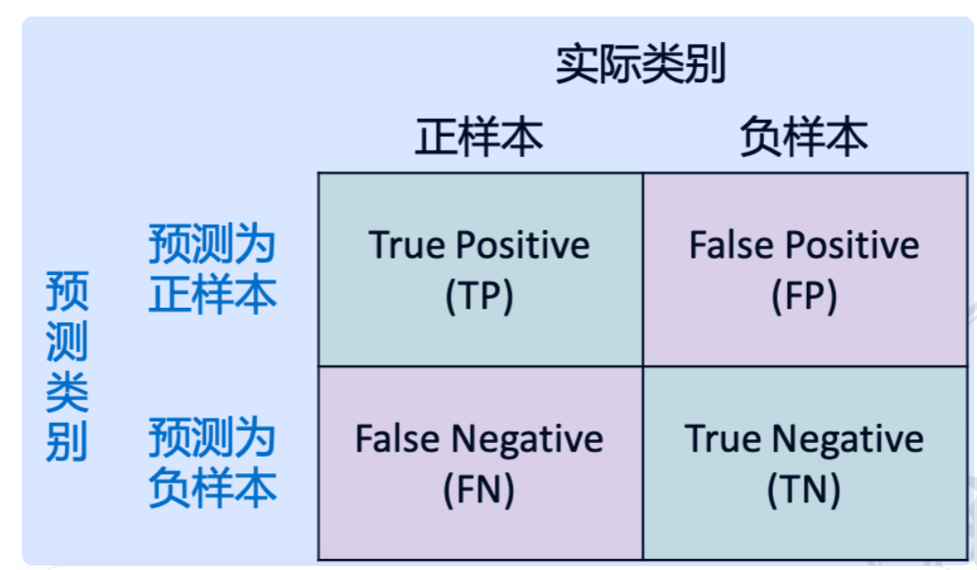
• Accuracy: the proportion of correctly predicted positive and negative samples among all samples $$Accuracy =\frac{TP+TN}{TP+FP+TN+FN}$$

Problem: in real speech detection scenarios, the distribution of speech and non-speech is often imbalanced. Most of the audio data may be non-speech, so predicting everything as non-speech still gives high accuracy.

Insight: this is a detection problem rather than a binary classification problem

• Recall / TPR (True Positive Rate): the proportion of all positive samples that are predicted correctly

  $$Precision =\frac{TP}{TP+FP}, \quad Recall =\frac{TP}{TP+FN}$$

• score: the (weighted) harmonic mean of precision and recall

  $$F_{\beta}=\left(1+\beta^{2}\right) \frac{ Precision × Recall }{\beta^{2} × Precision + Recall }$$

  where the value of β is chosen according to the relative importance of precision and recall in the evaluation; it is usually set to 1:

  $$F_{1}=\frac{2 × Precision × Recall }{ Precision + Recall }=\frac{2 × TP}{2 × TP+FP+FN}$$

  • Macro-averaging F1 score

    $$F_{macro }=\frac{1}{N} \sum_{n=1}^{N} F_{1, n}$$

  • Micro-averaging F1 score

    $$P_{micro }=\frac{\sum_{n=1}^{N} TP_{n}}{\sum_{n=1}^{N} TP_{n}+\sum_{n=1}^{N} FP_{n}}$$ $$R_{micro }=\frac{\sum_{n=1}^{N} TP_{n}}{\sum_{n=1}^{N} TP_{n}+\sum_{n=1}^{N} FN_{n}}$$ $$F_{micro }=\frac{2 × P_{micro } × R_{micro }}{P_{micro }+R_{micro }}$$

The macro average is an arithmetic mean and is strongly affected by extreme values; the micro average is a harmonic mean and is more sensitive to the data distribution

• ROC curve (Receiver Operating Characteristic curve): the curve formed by TPR (True Positive Rate) and FPR (False Positive Rate) at different thresholds TPR = TP TP + FN TNR = TN TN + FP,

  $$TNR=\frac{TN}{TN+FP}, FPR=1-TNR$$

• AUC (Area Under Curve): the area under the ROC curve

Lec12

n-gram Language Models

An n-gram language model is a statistical natural language processing model used to predict the probability of a text sequence. It models the regularities of language by computing the joint probability of word sequences, and is one of the core methods of early language modeling. Below is an analysis of its core concepts and applications:

1. Basic Concepts

• n-gram: a subsequence made up of n consecutive words.
  • Unigram (1-gram): a single word (e.g. “model”).
  • Bigram (2-gram): two adjacent words (e.g. “language model”).
  • Trigram (3-gram): three adjacent words (e.g. “natural language processing”).
• Markov assumption: assume the probability of the current word depends only on the previous n-1 words rather than on the entire history. For example:
  • Bigram model: $P(w_i | w_1, w_2, ..., w_{i-1}) \approx P(w_i | w_{i-1})$
  • Trigram model: $P(w_i | w_{i-2}, w_{i-1})$

2. Probability Computation

Count frequencies in a corpus using maximum likelihood estimation (MLE):

• Example: under a bigram model, $P(\text{model} | \text{language}) = \frac{\text{count of “language model”}}{\text{count of “language”}}$

Suppose that in the corpus:

• “I love” appears 100 times and “I love NLP” appears 30 times,
• then ( P(\text{NLP} | \text{love}) = \frac{30}{100} = 0.3 ).

When generating text, the next word (e.g. “NLP”) can be chosen according to these probabilities.

Branching Factor

• Branching factor: the number of possible values the current word can take given the previous n-1 words. The higher the branching factor, the more complex the model.
• Computation: $B(w_{i-1}) = \frac{\text{count}(w_{i-1})}{\text{count}(w_{i-1}, w_i)}$
• Example: in “I love natural language processing”, “I” may be followed by “love”, “like”, etc., giving a high branching factor; whereas if “I” can only be followed by “love”, the branching factor is low.

Perplexity

• Definition: perplexity is an evaluation metric for language models that expresses how “perplexed” the model is by the test set. The lower the value, the better the model.
• Computation: $PP(W) = 2^{-\frac{1}{N} \sum_{i=1}^{N} \log_2 P(w_i | w_{i-n+1}, ..., w_{i-1})}$
• Example: suppose the model assigns a probability of 0.01 to the sentence “I love natural language processing” and the sentence length is 5; then the perplexity is $PP = 2^{-\frac{1}{5} \log_2(0.01)} \approx 100$
• Perplexity can be infinite, because with sparse data some n-grams may never appear in the training set, giving them a probability of 0.

Lec13: Large Vocabulary Continuous Speech Recognition

Translated from the Chinese original.